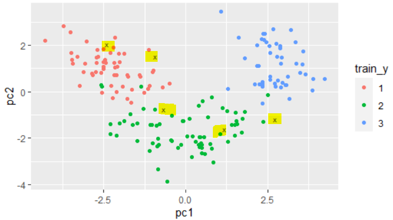
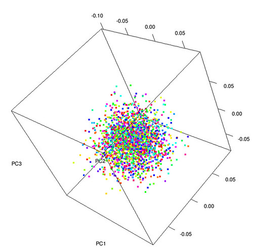
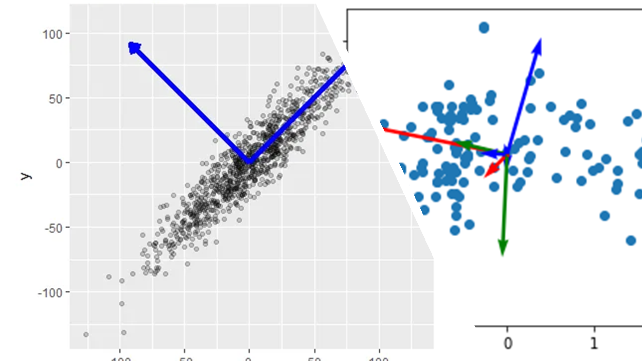
In this posting, there is WGS data, and after performing PCA, we will talk about the R code that draws PCplots based on PC values. First, before performing PCA, SNPs in LDs performed PCA based on data after performing Pruning process to remove LDs because SNPs in LDs cause problems during matrix calculation. First, the library used for data analysis is tidyverse. The tidyverse library called the ggplot() function to use in R.
/// R programming code library (tidyverse)

Next, the folder and the file name are specified. In data analysis, when the same code is turned for a plurality of situations, it is usually better to set up a pipeline to automatically store the results of the plurality of situations while changing the folder and the name for the input. For this reason, a library is put in the first paragraph and an input folder and a file name are put in the second paragraph. After that, the actual code is entered, and the substantial code part is not changed in the subsequent process once set.

/// /// R로그래r드_irdir_plink_prune=’plink_prune_father_prune’fname_vcf=’vcfnames/father_vcfname.txt’fname_pheno=’phenotype/pheno_father_standard.csv’fname_new=’phenotype/pheno_father_whiteonly_standard.csv’fname_standard=’phenotype/phather_whiteonly_standard.csv’pheno=’phather’

As can be seen from the code above, data obtained by merging the vcf file for each chromosome are secured, and if there is a file corresponding to the phenotype and a file to be used in covariates, the file can be defined. A variable storing position information of the eigenvalues and eigenvector values obtained as a result of PCA is assigned.

/// // <\FILE=paste0(dir_plink_prune, ‘/All’) pca=read. Table (paste0(FILE, ‘).envec’) enval=scan(paste0(FILE,’)).”Specific”)

/// // <\FILE=paste0(dir_plink_prune, ‘/All’) pca=read. Table (paste0(FILE, ‘).envec’) enval=scan(paste0(FILE,’)).”Specific”)/// R programming code pca<-pca[,-1]And I want to name each column. Here, since the first column is information for each sample, a character string ind is put in, and after that, a name is given from the PC1 to the last PC. However, you only have to look carefully at the part where you index using the size of the column using the ncol() function. Also, let’s use this to check the part of creating a PC name from the paste0() function./// R programming code colnames(pca)[1]<-‘ind’colnames(pca)[2:ncol(pca)]<-paste0(‘PC’,1:(ncol(pca)-1))Next, if there is information about race, the relevant data can be brought and then colored on the PC plot. The data I deal with has this information and takes this part, and if not, I can understand the structure of the population through clustering algorithms such as Random Forest. Therefore, the relevant race information is brought as follows./// R programming code df_race=read.delim(‘race/race_father.txt’)In the race data, the value of the column name new_ID becomes the ID of the sample. The sample ID in the pca data I brought before that is the name of the column ind, so you can merge the two. Merge it into the merge() function, but assign by.x and by.y respectively to apply different criteria to each data frame./// R __ rr f d dfmergeddf_race = merge (pca, df_race, by.x = ‘ind’, by.y = ‘new_ID’)In rare cases, race information may be NA or empty, and the following measures have been taken to exclude such cases. In other words, only non-empty cases, not NA, were taken as subsets()./// R’ ‘df_subset’ = subset (df_subset, !is.na (Ethnic).Category) and ethnicity.Category!=’)Next, create a new column called race, where Ethnic.Category takes only the information in the previous section. And the criterion for the front part is the string: the front part. To obtain this part of information, you must first use the strsplit() function to divide the string by : and take the previous value, which must be applied to all rows in the Ethnic.Category column of the data frame and brought into the vector. You can use the sapply() function to do it all at once./// /// R로_래r드코dfracedf_vpn$race=sapply(strsplit(df_merged$Ethnic)。Category, ‘:’), function (x)x[1])Now, we have collected information about race separately, but we can think of it as meaningful as a larger range of a larger range. Next, try to get their information about the not-stated part of the race that has similar traits to the main race. A reference value for this part is arbitrarily determined as 0.01 here, but this part will be upgraded using a clustering method./// R ththresr 코 ththresh=0.01df_diff=conversion (df_diff, race_differse=ifelse(race==”not mentioned”&-different<PC1&-different<PC2&PC1<threshold&PC2<threshold, “not mentioned”, race)/// R ththresr 코 ththresh=0.01df_diff=conversion (df_diff, race_differse=ifelse(race==”not mentioned”&-different<PC1&-different<PC2&PC1<threshold&PC2<threshold, “not mentioned”, race)/// /// /// R프로그래밍 코드df_merged = transform(df_merged, race_filtered = factor(ifelse(race_filtered %in%c(“Not Stated”, “Not Stated White”, “White”), race_filtered, “Others”), levels = c(“White”, “Not Stated White”, “Not Stated”, “Others”)))Now I created a variable that only collected the ID of the race of White and Not Stated White. This variable was taken in subset()./// /// /// R프로그래밍 코드filtered_ID=subset(df_subset,race_subset%in%c(“White”,”NotStatedWhite”))).indBased on the extracted ID, the phenotype and covariant data are called to take only the data belonging to the ID, and only the first value of the overlapping ID is taken and the rest is removed./// R ddf_r코 ddf_pheno=read.table(fname_pheno)df_tem=subset(df_pheno,V2% in %filtered_ID)df_whiteonly=df_tem [!duplicated(df_tem$V2),]A code above is filtered for phenotypes, and a code below is filtered for covariates./// R d df_r코 d df_summitiate=read.table(fname_summitiate) df_tem1 = subset (df_summitiate, V2% in %filtered_ID) df_whiteonly_cov = df_tem1 [!duplicated(df_tem1$V2),]Thus, the newly created phenotype and covariate data must be written as a new file. This part was done with the following code. Originally, it is a code that draws a PC plot, but since it is a part that proceeds based on the results of PCA and later, it was implemented with the same code./// R로그래밍드rwrite.table(df_whiteonly,fname_pheno_new,sep=’\t’,quote=F,row.names=F,col.names=F)write.table(df_whiteonly_cov,fname_col.namese,sep=’t)write.table(df_whiteonly$V2,f_vcf,colname=f,col.fFrom now on, we will draw PCAplot and distribution graphs using the ggplot() function. First of all, the ratio of the PC explaining the variance is calculated and flattened as follows. A data frame called pve is simply created so that PCs 1 to 20 appear on the x-axis, and the y-axis shows the specific gravity of dispersion described by each PC./// R p pver d datapve = data.frame(PC = 1:20, pve = eigenvalue /sum(valvalval)*100)pdf(00resultpca_result_,pheno, ‘_prune/PC_variance_,pheno, ‘.pdf’)a <-gg plot(pve,aes(PC,pve)+geom_bar(yabal’+aabal’+aabl’+a)<a)From now on, I will draw a PC plot, but if I draw PC1 vs PC2 first, I will be able to draw other PCs as long as I change the index.From now on, I will draw a PC plot, but if I draw PC1 vs PC2 first, I will be able to draw other PCs as long as I change the index./// R그래 ((r ppdf(00pcpca_result_,pheno,’_prune/PC_visual_,pheno,’.pdf’)b<-ggplot(df_pdf,aes(x=PC1,y=PC2,color=Pdf.Category)+geom_point(size=2)b<-b+code_(+++light{PC1<-pcs1+light{+light{+light{+light}+light}/// R그래 ((r ppdf(00pcpca_result_,pheno,’_prune/PC_visual_,pheno,’.pdf’)b<-ggplot(df_pdf,aes(x=PC1,y=PC2,color=Pdf.Category)+geom_point(size=2)b<-b+code_(+++light{PC1<-pcs1+light{+light{+light{+light}+light}
